11 Comparison of TransPropy with Other Tool Packages Using Ridge Plot
library(readr)
library(TransProR)
library(dplyr)
library(rlang)
library(linkET)
library(funkyheatmap)
library(tidyverse)
library(RColorBrewer)
library(ggalluvial)
library(tidyr)
library(tibble)
library(ggplot2)
library(ggridges)
library(reshape2)
library(gridExtra)
11.1 Finding the top three genes with the highest countdown: CFD, ANKRD35, ALOXE3
# Select all *countdown columns
test_formatted <- df_formatted[ ,c("id","deseq2countdown","edgeRcountdown","limmacountdown","outRstcountdown","TransPropycountdown")]

# Extract the rows where the values in the last column are greater than all previous columns
test_formatted1 <- test_formatted[apply(test_formatted[, -1], 1, function(row) all(row[length(row)] > row[1:(length(row)-1)])), ]
print(test_formatted1) # Show the total number of genes where the countdown is higher than that selected by the previous four methods

# Set the value of N
N <- 100  # Replace with your desired value
# Exclude the ID column from the comparison and find the rows where the value in the last column is greater than the maximum value of the previous columns by more than N
test_formatted2 <- test_formatted1[apply(test_formatted1[, -1], 1, function(row) max(row[1:(length(row)-1)]) + N < row[length(row)]), ]
# Display the result
print(test_formatted2)

# Sort by the difference between the last column and the maximum value of the previous columns, select the top N rows with the largest differences
N1 <- 3  # Replace with your desired value
# Calculate the difference and add it as a new column
test_formatted$Difference <- apply(test_formatted[, -1], 1, function(row) row[length(row)] - max(row[1:(length(row)-1)]))
# Sort the data frame by the Difference column in descending order
sorted_df <- test_formatted[order(-test_formatted$Difference), ]
# Select the top N rows
top_N1_rows <- head(sorted_df, N1)

# Display the result
print(top_N1_rows)
11.2 Bubble chart + stacked chart + bar chart + nested bar chart
test_formatted33 <- df_formatted[1:33 ,c("id","deseq2countdown","edgeRcountdown", "limmacountdown","outRstcountdown","TransPropycountdown")]
N1 <- 33  # Replace with your desired value
# Calculate the difference and add it as a new column
test_formatted33$Difference <- apply(test_formatted33[, -1], 1, function(row) row[length(row)] - max(row[1:(length(row)-1)]))
# Sort the data frame by the Difference column in descending order
sorted_df <- test_formatted33[order(-test_formatted33$Difference), ]
# Select the top N rows
top_N1_rows <- head(sorted_df, N1)
# Display the result
print(top_N1_rows)
top_N1_rows1 <- t(top_N1_rows[,c("id","deseq2countdown","edgeRcountdown","TransPropycountdown", "limmacountdown","outRstcountdown")])
colnames(top_N1_rows1) <- top_N1_rows1["id",]
top_N1_rows1 <- as.data.frame(top_N1_rows1[-1,])
top_N1_rows1$methods <- rownames(top_N1_rows1)
# rearrange
top_N1_rows1 <- top_N1_rows1[, c(ncol(top_N1_rows1), 1:(ncol(top_N1_rows1)-1))]
print(top_N1_rows1)
Convert data to long format
data_melt <- melt(top_N1_rows1, id.vars = "methods")
data_melt$value <- as.numeric(data_melt$value)
data_melt$methods <- factor(data_melt$methods, levels = unique(data_melt$methods))
levels(data_melt$methods)
##count
p1 <- ggplot(data_melt, aes( x = variable,y=value,fill = methods,
stratum = methods, alluvium = methods))+
geom_stratum(width = 0.5, color='white')+
geom_alluvium(alpha = 0.5,
width = 0.5,
curve_type = "linear")+
theme_minimal()+
theme(axis.text.x = element_text(angle = 45, hjust = 1),
panel.grid = element_blank())+
scale_fill_manual(values = c("#3273c1","#2b8f9a","#6e4ab4",
"#48884d","#a8a74e"))+
#scale_y_continuous(expand = c(0,0),name="",
#label=c("0%","25%","50%","75%","100%"))+
scale_x_discrete(expand = c(0,0),name="")+
theme(panel.background = element_blank(),
panel.grid = element_blank(),
axis.line = element_blank(),
axis.ticks.y = element_blank(),
axis.text = element_text(color="black",size=10),
axis.ticks.length.x = unit(0.1,"cm"),
plot.margin = margin(10, 10, 10, 10)
)
p1
down stacked chart
##percentage
# Calculate the total value for each variable
total_values <- data_melt %>%
  group_by(variable) %>%
  summarize(total = sum(value))

# Merge data frames to calculate percentages
data_melt <- data_melt %>%
  left_join(total_values, by = "variable") %>%
  mutate(percentage = (value / total) * 100)

ggplot(data_melt, aes(x = variable, y = percentage, fill = methods, stratum = methods, alluvium = methods)) +
  geom_stratum(width = 0.5, color = "white") +
  geom_alluvium(alpha = 0.5, width = 0.5, curve_type = "linear") +
  theme_minimal()+
  theme(axis.text.x = element_text(angle = 45, hjust = 1),
        panel.grid = element_blank())+
  theme(axis.text.x = element_text(angle = 45, hjust = 1),
        panel.grid = element_blank())+
  scale_fill_manual(values = c("#3273c1","#2b8f9a","#6e4ab4",
                               "#48884d","#a8a74e"))+
  #scale_y_continuous(expand = c(0,0),name="",
  #label=c("0%","25%","50%","75%","100%"))+
  scale_x_discrete(expand = c(0,0),name="")+
  theme(panel.background = element_blank(),
        panel.grid = element_blank(),
        axis.line = element_blank(),
        axis.ticks.y = element_blank(),
        axis.text = element_text(color="black",size=10),
        axis.ticks.length.x = unit(0.1,"cm"),
        plot.margin = margin(10, 10, 10, 10)
  )
p2 <- ggplot(data_melt, aes(x = variable, y = methods, size = value, color = methods)) +
geom_point(alpha = 0.7) +
scale_size_continuous(range = c(1, 10)) +
theme_minimal() +
theme(
panel.grid = element_blank(),
legend.position = "none",
axis.line = element_line(color = "black"),
axis.ticks = element_line(color = "black")
) +
theme_minimal()+
theme(axis.text.x = element_text(angle = 45, hjust = 1),
panel.grid = element_blank())+
scale_color_manual(values = c("#3273c1","#2b8f9a","#6e4ab4",
"#48884d","#a8a74e"))+
#scale_y_continuous(expand = c(0,0),name="",
#label=c("0%","25%","50%","75%","100%"))+
#scale_x_discrete(expand = c(0,0),name="")+
theme(panel.background = element_blank(),
panel.grid = element_blank(),
axis.line = element_blank(),
axis.ticks.y = element_blank(),
axis.text = element_text(color="black",size=10),
axis.ticks.length.x = unit(0.1,"cm"),
plot.margin = margin(10, 10, 10, 10)
)
#labs(x = "Time", y = "Cell Type", size = "Proportion (%)", color = "Cell Type")
p2
bubble
# bar chart
data_sums <- aggregate(value ~ methods, data = data_melt, sum)
data_sums$methods <- factor(data_sums$methods, levels = unique(data_sums$methods))
levels(data_sums$methods)

p3 <- ggplot(data_sums, aes(x = methods, y = value, fill = methods)) +
  geom_bar(stat = "identity") +
  coord_flip() +
  theme_minimal() +
  theme(
    panel.grid = element_blank(),
    legend.position = "none",
    axis.line = element_line(color = "black"),
    axis.ticks = element_line(color = "black")
  ) +
  theme_minimal()+
  theme(axis.text.x = element_text(angle = 45, hjust = 1),
        panel.grid = element_blank())+
  scale_fill_manual(values = c("#3273c1","#2b8f9a","#6e4ab4",
                                "#48884d","#a8a74e"))+
  #scale_y_continuous(expand = c(0,0),name="",
  #label=c("0%","25%","50%","75%","100%"))+
  scale_x_discrete(expand = c(0,0),name="")+
  theme(panel.background = element_blank(),
        panel.grid = element_blank(),
        axis.line = element_blank(),
        axis.ticks.y = element_blank(),
        axis.text = element_text(color="black",size=10),
        axis.ticks.length.x = unit(0.1,"cm"),
        plot.margin = margin(10, 10, 10, 10)
  )
  #labs(y = "Proportion (%)", fill = "Cell Type", x = "Cell Type")

p3
bar
library(tidyverse)
library(ggtext)
library(ggrepel)
library(patchwork)
library(systemfonts)
library(dplyr)

# Retain only the TransPropy and Difference columns along with the id column
selected_columns <- sorted_df[, c("TransPropycountdown", "Difference")]

# Get the maximum value and its corresponding column position from the first four columns of TransPropy for each row
max_values <- apply(sorted_df[, 2:5], 1, max)  # Assuming the first four columns are columns 2 to 5
max_index <- apply(sorted_df[, 2:5], 1, which.max)

# Create a new dataframe that retains the maximum value among the first four columns, setting other values to 0
new_data <- sorted_df[, 2:5]
for(i in 1:nrow(new_data)) {
  new_data[i, ] <- ifelse(1:4 == max_index[i], new_data[i, ], 0)
}

# Add the id, TransPropy, and Difference columns back to the new dataframe
new_data <- cbind(sorted_df[, "id"], new_data, selected_columns)

# Display the result
print(new_data)

# Rename the first column of the new dataframe to id
colnames(new_data)[1] <- "id"

new_data$id <- factor(new_data$id, levels = unique(new_data$id))
new_data$color1 <- "TransProPy"  # Add a pseudo-variable
new_data %>%
  ggplot(aes(id, TransPropycountdown)) +
  geom_col(aes(fill = "TransProPy"), width = .85) +
  scale_fill_manual(values = c("TransProPy" = "#6d4cb1"), name = "Legend Title") +
  labs(y = "TransPropycountdown", x = "ID") +
  theme_minimal() +  # Use a simple theme
  theme(axis.text.x = element_text(angle = 45, hjust = 1),
        panel.grid = element_blank())

# Create the color2 column
new_data <- new_data %>%
  mutate(color2 = case_when(
    deseq2countdown != 0 ~ "#3773bd",
    edgeRcountdown != 0 ~ "#358e99",
    limmacountdown != 0 ~ "#4b8954",
    outRstcountdown != 0 ~ "#a8a75a",
    TRUE ~ NA_character_
  ))

# Create the fourmethods column with non-zero elements from the four columns
new_data <- new_data %>%
  mutate(fourmethods = case_when(
    deseq2countdown != 0 ~ deseq2countdown,
    edgeRcountdown != 0 ~ edgeRcountdown,
    limmacountdown != 0 ~ limmacountdown,
    outRstcountdown != 0 ~ outRstcountdown,
    TRUE ~ NA_real_
  ))

# Base bar plot
base_plot <- new_data %>%
  ggplot(aes(id, TransPropycountdown)) +
  geom_col(fill = "#6d4cb1", width = .85, alpha = 1) +  # Use fixed color, not mapped with aes
  labs(y = "TransPropycountdown", x = "ID") +
  theme_minimal() +
  theme(axis.text.x = element_text(angle = 45, hjust = 1),
        panel.grid = element_blank())

# Overlay bar plot with text labels
overlay_plot <- base_plot +
  geom_col(
    data = new_data %>% filter(!is.na(fourmethods)),
    aes(x = id, y = fourmethods, fill = color2),
    width = .4, alpha = 0.9
  ) +
  scale_fill_identity(name = "Method", guide = "legend", labels = c("edgeR", "limma", "outRst")) +
  guides(fill = guide_legend(title = "Method")) +

  # Add text labels to the base bar plot
  geom_text(
    data = new_data,
    aes(x = id, y = TransPropycountdown, label = TransPropycountdown),
    size = 4.3, nudge_y = 12, vjust = 0, color = "#6d4cb1", fontface = "bold"
  ) +

  # Add text labels to the overlay bar plot
  geom_text(
    data = new_data %>% filter(!is.na(fourmethods)),
    aes(x = id, y = fourmethods, label = fourmethods, color = color2),
    size = 4.3, nudge_y = 12, vjust = 0, fontface = "bold"
  ) +
  scale_color_identity()

# Display the overlay plot
print(overlay_plot)
overlay_plot1
# Prepare data, sort by positive then negative differences
new_data1 <- new_data %>%
  mutate(group = ifelse(Difference >= 0, "Positive", "Negative")) %>%
  arrange(desc(Difference)) %>%
  mutate(id = factor(id, levels = id))

# Plot line graph
difference_line <- new_data1 %>%
  ggplot(aes(x = id, y = Difference, group = 1)) +
  geom_line(aes(color = group), linewidth = 1) +
  geom_point(size = 4, aes(color = group), show.legend = FALSE) +
  theme_bw(base_size = 20) +
  theme(panel.grid = element_blank(),
        axis.text.x = element_text(angle = 60, size = 15, hjust = 1, vjust = 1)) +
  scale_color_manual(values = c("Positive" = "#6c4dac", "Negative" = "#beb8d7"))

# Display line graph
print(difference_line)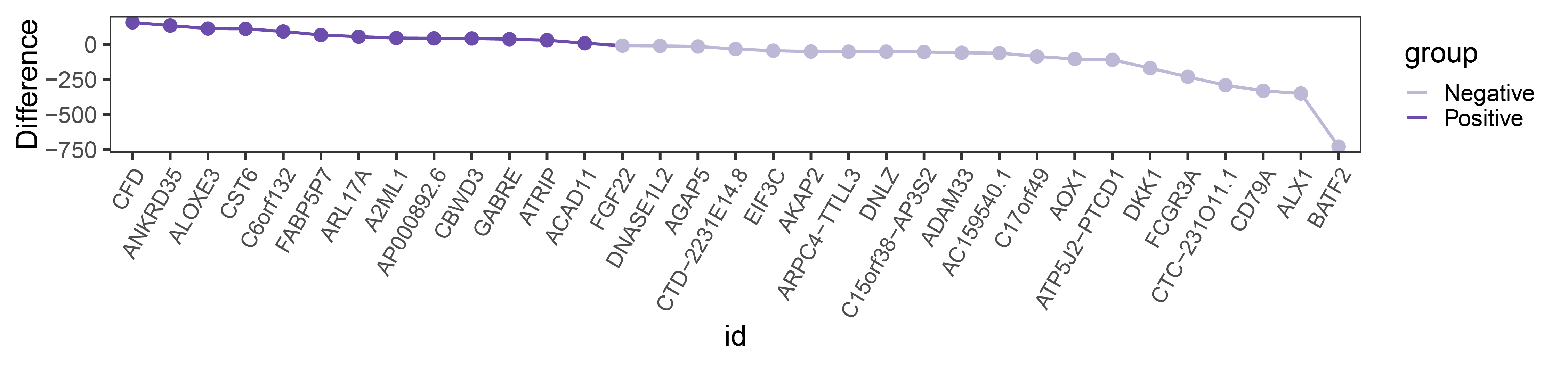
difference_line
# Prepare data, sort by positive then negative differences
new_data1 <- new_data %>%
  mutate(group = ifelse(Difference >= 0, "Positive", "Negative")) %>%
  arrange(desc(Difference)) %>%
  mutate(id = factor(id, levels = id))

# Plot bar graph
difference_bar <- new_data1 %>%
  ggplot(aes(x = id, y = Difference, fill = group)) +
  geom_col() +
  scale_fill_manual(values = c("Positive" = "#6c4dac", "Negative" = "#beb8d7"), name = "Difference Type") +
  theme_bw(base_size = 20) +
  theme(panel.grid = element_blank(),
        axis.text.x = element_text(angle = 60, size = 15, hjust = 1, vjust = 1)) +
  labs(y = "Difference", x = "ID")

# Display bar graph
print(difference_bar)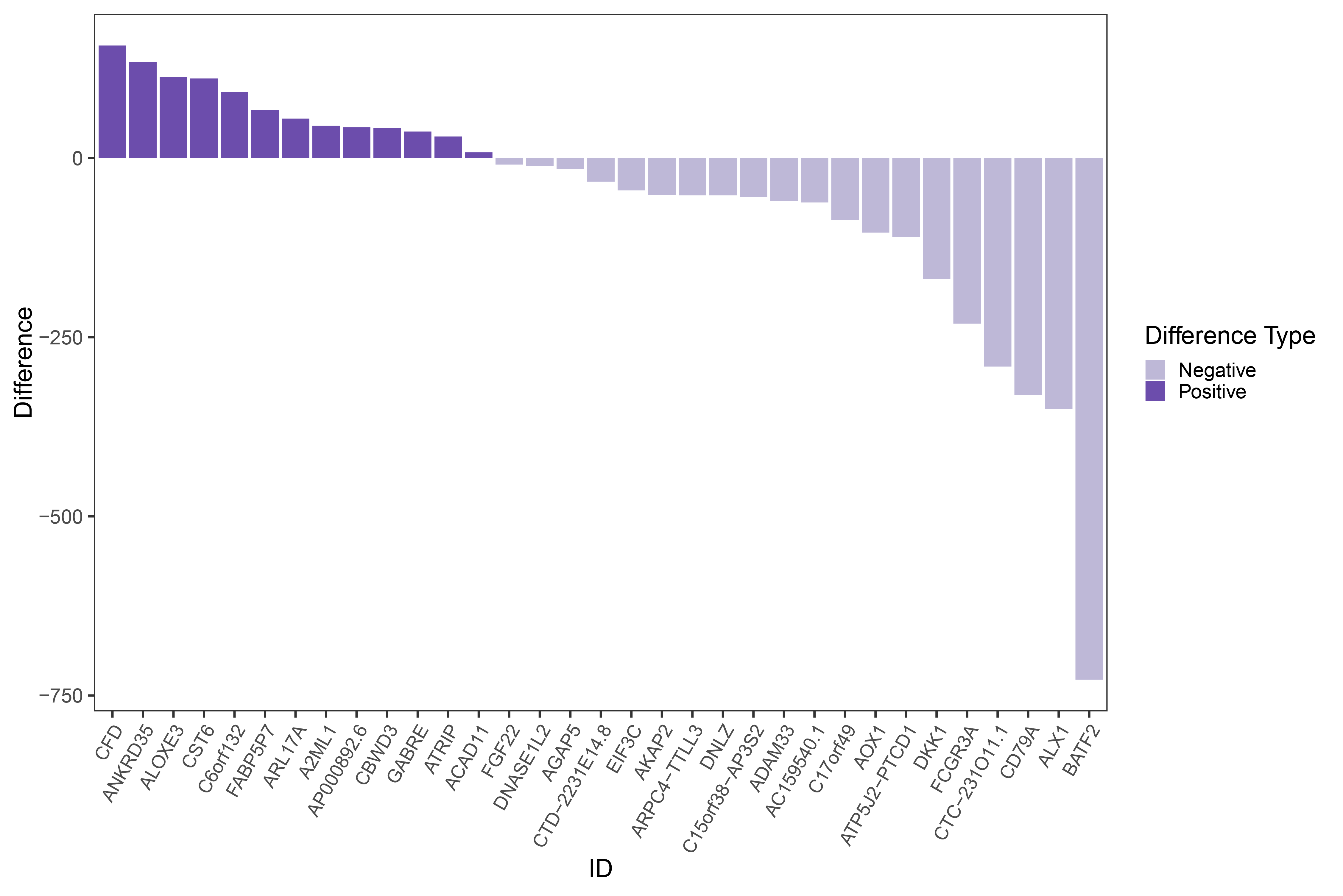
difference_bar
11.3 CFD
11.3.1 TRANSPROPY
#### TRANSPRO

# Set up the container for the final generated data
correlation <- data.frame()

TransPropy_CFD <- as.data.frame(TransPropy[,"CFD"])
colnames(TransPropy_CFD) <- c("CFD")

# Get the range for batch operations, which should be a vector
genelist <- colnames(TransPropy)

# Start the for loop, exporting data to the container
gene <- "CFD"
genedata <- as.numeric(TransPropy[,gene])

for(i in 1:length(genelist)) {
  # 1. Indicate progress
  print(i)
  # 2. Compute correlation
  dd <- cor.test(genedata, as.numeric(TransPropy[,i]), method="spearman")
  # 3. Fill in the data
  correlation[i,1] <- gene
  correlation[i,2] <- genelist[i]
  correlation[i,3] <- dd$estimate
  correlation[i,4] <- dd$p.value
}

colnames(correlation) <- c("gene1", "gene2", "cor", "p.value")
class(correlation)

correlation <- na.omit(correlation)
correlation_TransPropy_CFD <- correlation

# write.table(correlation_TransPropy_CFD, file="correlation_TransPropy_CFD.csv", sep=",", row.names=TRUE)

N <- 0.5 # Set the threshold to 0.5, for example
# Calculate the number of rows where the absolute value of 'cor' is greater than N
TransPropycount_CFD <- sum(abs(correlation_TransPropy_CFD$cor) > N)

# Print results
TransPropycountup_CFD <- sum(correlation_TransPropy_CFD$cor > N)
TransPropycountdown_CFD <- sum(correlation_TransPropy_CFD$cor < -N)
print(paste("TransPropycount_CFD:", TransPropycount_CFD,
            "TransPropycountup_CFD:", TransPropycountup_CFD,
            "TransPropycountdown_CFD:", TransPropycountdown_CFD))
11.3.2 DESEQ2
# Set up the container for the final generated data
correlation <- data.frame()

# Get the range for batch operations, which should be a vector
genelist <- colnames(deseq2)

# Start the for loop, exporting data to the container
gene <- "CFD"
genedata <- as.numeric(deseq2[,gene])

for(i in 1:length(genelist)) {
  # 1. Indicate progress
  print(i)
  # 2. Compute correlation
  dd <- cor.test(genedata, as.numeric(deseq2[,i]), method="spearman")
  # 3. Fill in the data
  correlation[i,1] <- gene
  correlation[i,2] <- genelist[i]
  correlation[i,3] <- dd$estimate
  correlation[i,4] <- dd$p.value
}

colnames(correlation) <- c("gene1", "gene2", "cor", "p.value")
class(correlation)

correlation <- na.omit(correlation)
correlation_deseq2_CFD <- correlation

# write.table(correlation_deseq2_CFD, file="correlation_deseq2_CFD.csv", sep=",", row.names=TRUE)

N <- 0.5 # Set the threshold to 0.5, for example
# Calculate the number of rows where the absolute value of 'cor' is greater than N
deseq2count_CFD <- sum(abs(correlation_deseq2_CFD$cor) > N)

# Print results
deseq2countup_CFD <- sum(correlation_deseq2_CFD$cor > N)
deseq2countdown_CFD <- sum(correlation_deseq2_CFD$cor < -N)
print(paste("deseq2count_CFD:", deseq2count_CFD,
            "deseq2countup_CFD:", deseq2countup_CFD,
            "deseq2countdown_CFD:", deseq2countdown_CFD))
11.3.3 edgeR
# Set up the container for the final generated data
correlation <- data.frame()

# Get the range for batch operations, which should be a vector
genelist <- colnames(edgeR)

# Start the for loop, exporting data to the container
gene <- "CFD"
genedata <- as.numeric(edgeR[,gene])

for(i in 1:length(genelist)) {
  # 1. Indicate progress
  print(i)
  # 2. Compute correlation
  dd <- cor.test(genedata, as.numeric(edgeR[,i]), method="spearman")
  # 3. Fill in the data
  correlation[i,1] <- gene
  correlation[i,2] <- genelist[i]
  correlation[i,3] <- dd$estimate
  correlation[i,4] <- dd$p.value
}

colnames(correlation) <- c("gene1", "gene2", "cor", "p.value")
class(correlation)

correlation <- na.omit(correlation)
correlation_edgeR_CFD <- correlation

# write.table(correlation_edgeR_CFD, file="correlation_edgeR_CFD.csv", sep=",", row.names=TRUE)

N <- 0.5 # Set the threshold to 0.5, for example
# Calculate the number of rows where the absolute value of 'cor' is greater than N
edgeRcount_CFD <- sum(abs(correlation_edgeR_CFD$cor) > N)

# Print results
edgeRcountup_CFD <- sum(correlation_edgeR_CFD$cor > N)
edgeRcountdown_CFD <- sum(correlation_edgeR_CFD$cor < -N)
print(paste("edgeRcount_CFD:", edgeRcount_CFD,
            "edgeRcountup_CFD:", edgeRcountup_CFD,
            "edgeRcountdown_CFD:", edgeRcountdown_CFD))
11.3.4 limma
# Set up the container for the final generated data
correlation <- data.frame()

# Get the range for batch operations, which should be a vector
genelist <- colnames(limma)

# Start the for loop, exporting data to the container
gene <- "CFD"
genedata <- as.numeric(limma[,gene])

for(i in 1:length(genelist)) {
  # 1. Indicate progress
  print(i)
  # 2. Compute correlation
  dd <- cor.test(genedata, as.numeric(limma[,i]), method="spearman")
  # 3. Fill in the data
  correlation[i,1] <- gene
  correlation[i,2] <- genelist[i]
  correlation[i,3] <- dd$estimate
  correlation[i,4] <- dd$p.value
}

colnames(correlation) <- c("gene1", "gene2", "cor", "p.value")
class(correlation)

correlation <- na.omit(correlation)
correlation_limma_CFD <- correlation

# write.table(correlation_limma_CFD, file="correlation_limma_CFD.csv", sep=",", row.names=TRUE)

N <- 0.5 # Set the threshold to 0.5, for example
# Calculate the number of rows where the absolute value of 'cor' is greater than N
limmacount_CFD <- sum(abs(correlation_limma_CFD$cor) > N)

# Print results
limmacountup_CFD <- sum(correlation_limma_CFD$cor > N)
limmacountdown_CFD <- sum(correlation_limma_CFD$cor < -N)
print(paste("limmacount_CFD:", limmacount_CFD,
            "limmacountup_CFD:", limmacountup_CFD,
            "limmacountdown_CFD:", limmacountdown_CFD))
11.3.5 outRst
# Set up the container for the final generated data
correlation <- data.frame()

# Get the range for batch operations, which should be a vector
genelist <- colnames(outRst)

# Start the for loop, exporting data to the container
gene <- "CFD"
genedata <- as.numeric(outRst[,gene])

for(i in 1:length(genelist)) {
  # 1. Indicate progress
  print(i)
  # 2. Compute correlation
  dd <- cor.test(genedata, as.numeric(outRst[,i]), method="spearman")
  # 3. Fill in the data
  correlation[i,1] <- gene
  correlation[i,2] <- genelist[i]
  correlation[i,3] <- dd$estimate
  correlation[i,4] <- dd$p.value
}

colnames(correlation) <- c("gene1", "gene2", "cor", "p.value")
class(correlation)

correlation <- na.omit(correlation)
correlation_outRst_CFD <- correlation

# write.table(correlation_outRst_CFD, file="correlation_outRst_CFD.csv", sep=",", row.names=TRUE)

N <- 0.5 # Set the threshold to 0.5, for example
# Calculate the number of rows where the absolute value of 'cor' is greater than N
outRstcount_CFD <- sum(abs(correlation_outRst_CFD$cor) > N)

# Print results
outRstcountup_CFD <- sum(correlation_outRst_CFD$cor > N)
outRstcountdown_CFD <- sum(correlation_outRst_CFD$cor < -N)
print(paste("outRstcount_CFD:", outRstcount_CFD,
            "outRstcountup_CFD:", outRstcountup_CFD,
            "outRstcountdown_CFD:", outRstcountdown_CFD))
11.4 ANKRD35
11.4.1 TRANSPROPY
# Set the container to store the final generated data
correlation <- data.frame()

# Get the range for batch processing, which should be a vector
genelist <- colnames(TransPropy)

# Start the for loop, exporting data to the container
gene <- "ANKRD35"
genedata <- as.numeric(TransPropy[, gene])

for (i in 1:length(genelist)) {
  # 1. Indicate progress
  print(i)
  # 2. Calculate correlation
  dd = cor.test(genedata, as.numeric(TransPropy[, i]), method="spearman")
  # 3. Fill the container
  correlation[i, 1] = gene
  correlation[i, 2] = genelist[i]
  correlation[i, 3] = dd$estimate
  correlation[i, 4] = dd$p.value
}

colnames(correlation) <- c("gene1", "gene2", "cor", "p.value")
class(correlation)

correlation = na.omit(correlation)
correlation_TransPropy_ANKRD35 <- correlation

# write.table(correlation_TransPropy_ANKRD35, file="correlation_TransPropy_ANKRD35.csv", sep=",", row.names=T)

N <- 0.5  # Set threshold to 0.5
TransPropycount_ANKRD35 <- sum(abs(correlation_TransPropy_ANKRD35$cor) > N)

TransPropycountup_ANKRD35 <- sum(correlation_TransPropy_ANKRD35$cor > N)
TransPropycountdown_ANKRD35 <- sum(correlation_TransPropy_ANKRD35$cor < -N)
print(paste("TransPropycount_ANKRD35:", TransPropycount_ANKRD35,
            "TransPropycountup_ANKRD35:", TransPropycountup_ANKRD35,
            "TransPropycountdown_ANKRD35:", TransPropycountdown_ANKRD35))
11.4.2 DESEQ2
# Set the container to store the final generated data
correlation <- data.frame()

# Get the range for batch processing, which should be a vector
genelist <- colnames(deseq2)

# Start the for loop, exporting data to the container
gene <- "ANKRD35"
genedata <- as.numeric(deseq2[, gene])

for (i in 1:length(genelist)) {
  # 1. Indicate progress
  print(i)
  # 2. Calculate correlation
  dd = cor.test(genedata, as.numeric(deseq2[, i]), method="spearman")
  # 3. Fill the container
  correlation[i, 1] = gene
  correlation[i, 2] = genelist[i]
  correlation[i, 3] = dd$estimate
  correlation[i, 4] = dd$p.value
}

colnames(correlation) <- c("gene1", "gene2", "cor", "p.value")
class(correlation)

correlation = na.omit(correlation)
correlation_deseq2_ANKRD35 <- correlation

# write.table(correlation_deseq2_ANKRD35, file="correlation_deseq2_ANKRD35.csv", sep=",", row.names=T)

N <- 0.5  # Set threshold to 0.5
deseq2count_ANKRD35 <- sum(abs(correlation_deseq2_ANKRD35$cor) > N)

deseq2countup_ANKRD35 <- sum(correlation_deseq2_ANKRD35$cor > N)
deseq2countdown_ANKRD35 <- sum(correlation_deseq2_ANKRD35$cor < -N)
print(paste("deseq2count_ANKRD35:", deseq2count_ANKRD35,
            "deseq2countup_ANKRD35:", deseq2countup_ANKRD35,
            "deseq2countdown_ANKRD35:", deseq2countdown_ANKRD35))
11.4.3 edgeR
# Set the container to store the final generated data
correlation <- data.frame()

# Get the range for batch processing, which should be a vector
genelist <- colnames(edgeR)

# Start the for loop, exporting data to the container
gene <- "ANKRD35"
genedata <- as.numeric(edgeR[, gene])

for (i in 1:length(genelist)) {
  # 1. Indicate progress
  print(i)
  # 2. Calculate correlation
  dd = cor.test(genedata, as.numeric(edgeR[, i]), method="spearman")
  # 3. Fill the container
  correlation[i, 1] = gene
  correlation[i, 2] = genelist[i]
  correlation[i, 3] = dd$estimate
  correlation[i, 4] = dd$p.value
}

colnames(correlation) <- c("gene1", "gene2", "cor", "p.value")
class(correlation)

correlation = na.omit(correlation)
correlation_edgeR_ANKRD35 <- correlation

# write.table(correlation_edgeR_ANKRD35, file="correlation_edgeR_ANKRD35.csv", sep=",", row.names=T)

N <- 0.5  # Set threshold to 0.5
edgeRcount_ANKRD35 <- sum(abs(correlation_edgeR_ANKRD35$cor) > N)

edgeRcountup_ANKRD35 <- sum(correlation_edgeR_ANKRD35$cor > N)
edgeRcountdown_ANKRD35 <- sum(correlation_edgeR_ANKRD35$cor < -N)
print(paste("edgeRcount_ANKRD35:", edgeRcount_ANKRD35,
            "edgeRcountup_ANKRD35:", edgeRcountup_ANKRD35,
            "edgeRcountdown_ANKRD35:", edgeRcountdown_ANKRD35))
11.4.4 limma
# Set the container to store the final generated data
correlation <- data.frame()
# Get the range for batch processing, which should be a vector
genelist <- colnames(limma)
# Start the for loop, exporting data to the container
gene <- "ANKRD35"
genedata <- as.numeric(limma[, gene])

for (i in 1:length(genelist)) {
  # 1. Indicate progress
  print(i)
  # 2. Calculate correlation
  dd = cor.test(genedata, as.numeric(limma[, i]), method="spearman")
  # 3. Fill the container
  correlation[i, 1] = gene
  correlation[i, 2] = genelist[i]
  correlation[i, 3] = dd$estimate
  correlation[i, 4] = dd$p.value
}

colnames(correlation) <- c("gene1", "gene2", "cor", "p.value")
class(correlation)

correlation = na.omit(correlation)
correlation_limma_ANKRD35 <- correlation

# write.table(correlation_limma_ANKRD35, file="correlation_limma_ANKRD35.csv", sep=",", row.names=T)

N <- 0.5  # Set threshold to 0.5
limmacount_ANKRD35 <- sum(abs(correlation_limma_ANKRD35$cor) > N)

limmacountup_ANKRD35 <- sum(correlation_limma_ANKRD35$cor > N)
limmacountdown_ANKRD35 <- sum(correlation_limma_ANKRD35$cor < -N)
print(paste("limmacount_ANKRD35:", limmacount_ANKRD35,
            "limmacountup_ANKRD35:", limmacountup_ANKRD35,
            "limmacountdown_ANKRD35:", limmacountdown_ANKRD35))
11.4.5 outRst
# Set the container to store the final generated data
correlation <- data.frame()
# Get the range for batch processing, which should be a vector
genelist <- colnames(outRst)
# Start the for loop, exporting data to the container
gene <- "ANKRD35"
genedata <- as.numeric(outRst[, gene])

for (i in 1:length(genelist)) {
  # 1. Indicate progress
  print(i)
  # 2. Calculate correlation
  dd = cor.test(genedata, as.numeric(outRst[, i]), method="spearman")
  # 3. Fill the container
  correlation[i, 1] = gene
  correlation[i, 2] = genelist[i]
  correlation[i, 3] = dd$estimate
  correlation[i, 4] = dd$p.value
}

colnames(correlation) <- c("gene1", "gene2", "cor", "p.value")
class(correlation)

correlation = na.omit(correlation)
correlation_outRst_ANKRD35 <- correlation

# write.table(correlation_outRst_ANKRD35, file="correlation_outRst_ANKRD35.csv", sep=",", row.names=T)

N <- 0.5  # Set threshold to 0.5
outRstcount_ANKRD35 <- sum(abs(correlation_outRst_ANKRD35$cor) > N)

outRstcountup_ANKRD35 <- sum(correlation_outRst_ANKRD35$cor > N)
outRstcountdown_ANKRD35 <- sum(correlation_outRst_ANKRD35$cor < -N)
print(paste("outRstcount_ANKRD35:", outRstcount_ANKRD35,
            "outRstcountup_ANKRD35:", outRstcountup_ANKRD35,
            "outRstcountdown_ANKRD35:", outRstcountdown_ANKRD35))
11.5 ALOXE3
11.5.1 TRANSPROPY
# Set the container to store the final generated data
correlation <- data.frame()
# Get the range for batch processing, which should be a vector
genelist <- colnames(TransPropy)
# Start the for loop, exporting data to the container
gene <- "ALOXE3"
genedata <- as.numeric(TransPropy[, gene])

for (i in 1:length(genelist)) {
  # 1. Indicate progress
  print(i)
  # 2. Calculate correlation
  dd = cor.test(genedata, as.numeric(TransPropy[, i]), method="spearman")
  # 3. Fill the container
  correlation[i, 1] = gene
  correlation[i, 2] = genelist[i]
  correlation[i, 3] = dd$estimate
  correlation[i, 4] = dd$p.value
}

colnames(correlation) <- c("gene1", "gene2", "cor", "p.value")
class(correlation)

correlation = na.omit(correlation)
correlation_TransPropy_ALOXE3 <- correlation

# write.table(correlation_TransPropy_ALOXE3, file="correlation_TransPropy_ALOXE3.csv", sep=",", row.names=T)

N <- 0.5  # Set threshold to 0.5
TransPropycount_ALOXE3 <- sum(abs(correlation_TransPropy_ALOXE3$cor) > N)

TransPropycountup_ALOXE3 <- sum(correlation_TransPropy_ALOXE3$cor > N)
TransPropycountdown_ALOXE3 <- sum(correlation_TransPropy_ALOXE3$cor < -N)
print(paste("TransPropycount_ALOXE3:", TransPropycount_ALOXE3,
            "TransPropycountup_ALOXE3:", TransPropycountup_ALOXE3,
            "TransPropycountdown_ALOXE3:", TransPropycountdown_ALOXE3))
11.5.2 DESEQ2
# Set the container to store the final generated data
correlation <- data.frame()
# Get the range for batch processing, which should be a vector
genelist <- colnames(deseq2)
# Start the for loop, exporting data to the container
gene <- "ALOXE3"
genedata <- as.numeric(deseq2[, gene])

for (i in 1:length(genelist)) {
  # 1. Indicate progress
  print(i)
  # 2. Calculate correlation
  dd = cor.test(genedata, as.numeric(deseq2[, i]), method="spearman")
  # 3. Fill the container
  correlation[i, 1] = gene
  correlation[i, 2] = genelist[i]
  correlation[i, 3] = dd$estimate
  correlation[i, 4] = dd$p.value
}

colnames(correlation) <- c("gene1", "gene2", "cor", "p.value")
class(correlation)

correlation = na.omit(correlation)
correlation_deseq2_ALOXE3 <- correlation

# write.table(correlation_deseq2_ALOXE3, file="correlation_deseq2_ALOXE3.csv", sep=",", row.names=T)

N <- 0.5  # Set threshold to 0.5
deseq2count_ALOXE3 <- sum(abs(correlation_deseq2_ALOXE3$cor) > N)

deseq2countup_ALOXE3 <- sum(correlation_deseq2_ALOXE3$cor > N)
deseq2countdown_ALOXE3 <- sum(correlation_deseq2_ALOXE3$cor < -N)
print(paste("deseq2count_ALOXE3:", deseq2count_ALOXE3,
            "deseq2countup_ALOXE3:", deseq2countup_ALOXE3,
            "deseq2countdown_ALOXE3:", deseq2countdown_ALOXE3))
11.5.3 edgeR
# Set the container to store the final generated data
correlation <- data.frame()
# Get the range for batch processing, which should be a vector
genelist <- colnames(edgeR)
# Start the for loop, exporting data to the container
gene <- "ALOXE3"
genedata <- as.numeric(edgeR[, gene])

for (i in 1:length(genelist)) {
  # 1. Indicate progress
  print(i)
  # 2. Calculate correlation
  dd = cor.test(genedata, as.numeric(edgeR[, i]), method="spearman")
  # 3. Fill the container
  correlation[i, 1] = gene
  correlation[i, 2] = genelist[i]
  correlation[i, 3] = dd$estimate
  correlation[i, 4] = dd$p.value
}

colnames(correlation) <- c("gene1", "gene2", "cor", "p.value")
class(correlation)

correlation = na.omit(correlation)
correlation_edgeR_ALOXE3 <- correlation

# write.table(correlation_edgeR_ALOXE3, file="correlation_edgeR_ALOXE3.csv", sep=",", row.names=T)

N <- 0.5  # Set threshold to 0.5
edgeRcount_ALOXE3 <- sum(abs(correlation_edgeR_ALOXE3$cor) > N)

edgeRcountup_ALOXE3 <- sum(correlation_edgeR_ALOXE3$cor > N)
edgeRcountdown_ALOXE3 <- sum(correlation_edgeR_ALOXE3$cor < -N)
print(paste("edgeRcount_ALOXE3:", edgeRcount_ALOXE3,
            "edgeRcountup_ALOXE3:", edgeRcountup_ALOXE3,
            "edgeRcountdown_ALOXE3:", edgeRcountdown_ALOXE3))
11.5.4 limma
# Set the container to store the final generated data
correlation <- data.frame()
# Get the range for batch processing, which should be a vector
genelist <- colnames(limma)
# Start the for loop, exporting data to the container
gene <- "ALOXE3"
genedata <- as.numeric(limma[, gene])

for (i in 1:length(genelist)) {
  # 1. Indicate progress
  print(i)
  # 2. Calculate correlation
  dd = cor.test(genedata, as.numeric(limma[, i]), method="spearman")
  # 3. Fill the container
  correlation[i, 1] = gene
  correlation[i, 2] = genelist[i]
  correlation[i, 3] = dd$estimate
  correlation[i, 4] = dd$p.value
}

colnames(correlation) <- c("gene1", "gene2", "cor", "p.value")
class(correlation)

correlation = na.omit(correlation)
correlation_limma_ALOXE3 <- correlation

# write.table(correlation_limma_ALOXE3, file="correlation_limma_ALOXE3.csv", sep=",", row.names=T)

N <- 0.5  # Set threshold to 0.5
limmacount_ALOXE3 <- sum(abs(correlation_limma_ALOXE3$cor) > N)

limmacountup_ALOXE3 <- sum(correlation_limma_ALOXE3$cor > N)
limmacountdown_ALOXE3 <- sum(correlation_limma_ALOXE3$cor < -N)
print(paste("limmacount_ALOXE3:", limmacount_ALOXE3,
            "limmacountup_ALOXE3:", limmacountup_ALOXE3,
            "limmacountdown_ALOXE3:", limmacountdown_ALOXE3))
11.5.5 outRst
# Set the container to store the final generated data
correlation <- data.frame()
# Get the range for batch processing, which should be a vector
genelist <- colnames(outRst)
# Start the for loop, exporting data to the container
gene <- "ALOXE3"
genedata <- as.numeric(outRst[, gene])

for (i in 1:length(genelist)) {
  # 1. Indicate progress
  print(i)
  # 2. Calculate correlation
  dd = cor.test(genedata, as.numeric(outRst[, i]), method="spearman")
  # 3. Fill the container
  correlation[i, 1] = gene
  correlation[i, 2] = genelist[i]
  correlation[i, 3] = dd$estimate
  correlation[i, 4] = dd$p.value
}

colnames(correlation) <- c("gene1", "gene2", "cor", "p.value")
class(correlation)

correlation = na.omit(correlation)
correlation_outRst_ALOXE3 <- correlation

# write.table(correlation_outRst_ALOXE3, file="correlation_outRst_ALOXE3.csv", sep=",", row.names=T)

N <- 0.5  # Set threshold to 0.5
outRstcount_ALOXE3 <- sum(abs(correlation_outRst_ALOXE3$cor) > N)

outRstcountup_ALOXE3 <- sum(correlation_outRst_ALOXE3$cor > N)
outRstcountdown_ALOXE3 <- sum(correlation_outRst_ALOXE3$cor < -N)
print(paste("outRstcount_ALOXE3:", outRstcount_ALOXE3,
            "outRstcountup_ALOXE3:", outRstcountup_ALOXE3,
            "outRstcountdown_ALOXE3:", outRstcountdown_ALOXE3))
11.6 Creating a new column to mark the positive and negative correlations
# correlation_TransPropy_CFD
correlation_TransPropy_CFD$cor_type <- ifelse(correlation_TransPropy_CFD$cor > 0,
                                              "TransPropy_Positive", "TransPropy_Negative")
correlation_TransPropy_CFD$methods <- "TransPropy"

# correlation_deseq2_CFD
correlation_deseq2_CFD$cor_type <- ifelse(correlation_deseq2_CFD$cor > 0,
                                              "deseq2_Positive", "deseq2_Negative")
correlation_deseq2_CFD$methods <- "deseq2"

# correlation_edgeR_CFD
correlation_edgeR_CFD$cor_type <- ifelse(correlation_edgeR_CFD$cor > 0,
                                              "edgeR_Positive", "edgeR_Negative")
correlation_edgeR_CFD$methods <- "edgeR"

# correlation_limma_CFD
correlation_limma_CFD$cor_type <- ifelse(correlation_limma_CFD$cor > 0,
                                              "limma_Positive", "limma_Negative")
correlation_limma_CFD$methods <- "limma"

# correlation_outRst_CFD
correlation_outRst_CFD$cor_type <- ifelse(correlation_outRst_CFD$cor > 0,
                                              "outRst_Positive", "outRst_Negative")
correlation_outRst_CFD$methods <- "outRst"

combined_CFD <- rbind(correlation_TransPropy_CFD,
                      correlation_deseq2_CFD,
                      correlation_edgeR_CFD,
                      correlation_limma_CFD,
                      correlation_outRst_CFD)

# correlation_TransPropy_ANKRD35
correlation_TransPropy_ANKRD35$cor_type <- ifelse(correlation_TransPropy_ANKRD35$cor > 0,
                                              "TransPropy_Positive", "TransPropy_Negative")
correlation_TransPropy_ANKRD35$methods <- "TransPropy"

# correlation_deseq2_ANKRD35
correlation_deseq2_ANKRD35$cor_type <- ifelse(correlation_deseq2_ANKRD35$cor > 0,
                                              "deseq2_Positive", "deseq2_Negative")
correlation_deseq2_ANKRD35$methods <- "deseq2"

# correlation_edgeR_ANKRD35
correlation_edgeR_ANKRD35$cor_type <- ifelse(correlation_edgeR_ANKRD35$cor > 0,
                                              "edgeR_Positive", "edgeR_Negative")
correlation_edgeR_ANKRD35$methods <- "edgeR"

# correlation_limma_ANKRD35
correlation_limma_ANKRD35$cor_type <- ifelse(correlation_limma_ANKRD35$cor > 0,
                                              "limma_Positive", "limma_Negative")
correlation_limma_ANKRD35$methods <- "limma"

# correlation_outRst_ANKRD35
correlation_outRst_ANKRD35$cor_type <- ifelse(correlation_outRst_ANKRD35$cor > 0,
                                              "outRst_Positive", "outRst_Negative")
correlation_outRst_ANKRD35$methods <- "outRst"

combined_ANKRD35 <- rbind(correlation_TransPropy_ANKRD35,
                      correlation_deseq2_ANKRD35,
                      correlation_edgeR_ANKRD35,
                      correlation_limma_ANKRD35,
                      correlation_outRst_ANKRD35)

# correlation_TransPropy_ALOXE3
correlation_TransPropy_ALOXE3$cor_type <- ifelse(correlation_TransPropy_ALOXE3$cor > 0,
                                              "TransPropy_Positive", "TransPropy_Negative")
correlation_TransPropy_ALOXE3$methods <- "TransPropy"

# correlation_deseq2_ALOXE3
correlation_deseq2_ALOXE3$cor_type <- ifelse(correlation_deseq2_ALOXE3$cor > 0,
                                              "deseq2_Positive", "deseq2_Negative")
correlation_deseq2_ALOXE3$methods <- "deseq2"

# correlation_edgeR_ALOXE3
correlation_edgeR_ALOXE3$cor_type <- ifelse(correlation_edgeR_ALOXE3$cor > 0,
                                              "edgeR_Positive", "edgeR_Negative")
correlation_edgeR_ALOXE3$methods <- "edgeR"

# correlation_limma_ALOXE3
correlation_limma_ALOXE3$cor_type <- ifelse(correlation_limma_ALOXE3$cor > 0,
                                              "limma_Positive", "limma_Negative")
correlation_limma_ALOXE3$methods <- "limma"

# correlation_outRst_ALOXE3
correlation_outRst_ALOXE3$cor_type <- ifelse(correlation_outRst_ALOXE3$cor > 0,
                                              "outRst_Positive", "outRst_Negative")
correlation_outRst_ALOXE3$methods <- "outRst"

combined_ALOXE3 <- rbind(correlation_TransPropy_ALOXE3,
                          correlation_deseq2_ALOXE3,
                          correlation_edgeR_ALOXE3,
                          correlation_limma_ALOXE3,
                          correlation_outRst_ALOXE3)
11.7 CFD Ridge Plot
# Define colors for CFD Gene
colors <- rev(c("#ee3e42", "#25789a", "#e96e29", "#547089", "#ee8f1d", "#488a87", "#ee7f46", "#41a286", "#efbe4d", "#8ab569"))

# Plot Ridge Plot for CFD Gene
ggplot(combined_CFD, aes(x = cor, y = methods, fill = cor_type)) +
  geom_density_ridges(
    alpha = 0.7,
    color = 'white',
    scale = 1,  # Adjust overlap degree, scale = 1 just touches the baseline, larger values increase overlap
    rel_min_height = 0.01,  # Tail trimming, larger values trim more
    quantile_lines = TRUE,
    quantiles = 2,
    linewidth = 1
  ) +
  scale_fill_manual(values = colors) +
  labs(
    title = "Ridge Plot for Positive and Negative Correlations of CFD Gene",
    x = "Correlation",
    y = "CFD"
  ) +
  theme(
    axis.text.x = element_text(angle = 90, hjust = 1)
  ) +
  geom_vline(
    xintercept = c(-0.5, 0.5),
    linewidth = 1,
    color = 'grey50',
    lty = 'dashed',
    alpha = 0.3
  ) +
  geom_vline(
    xintercept = c(-1, 0, 1),
    linewidth = 0.4,
    color = 'grey',
    lty = 'dashed',
    alpha = 0.8
  ) +
  theme_classic() +
  scale_y_discrete(expand = c(0,0)) +
  theme_minimal() +
  theme(
    panel.grid = element_blank(),
    # axis.text.y = element_blank(),
    legend.title = element_blank()
  )
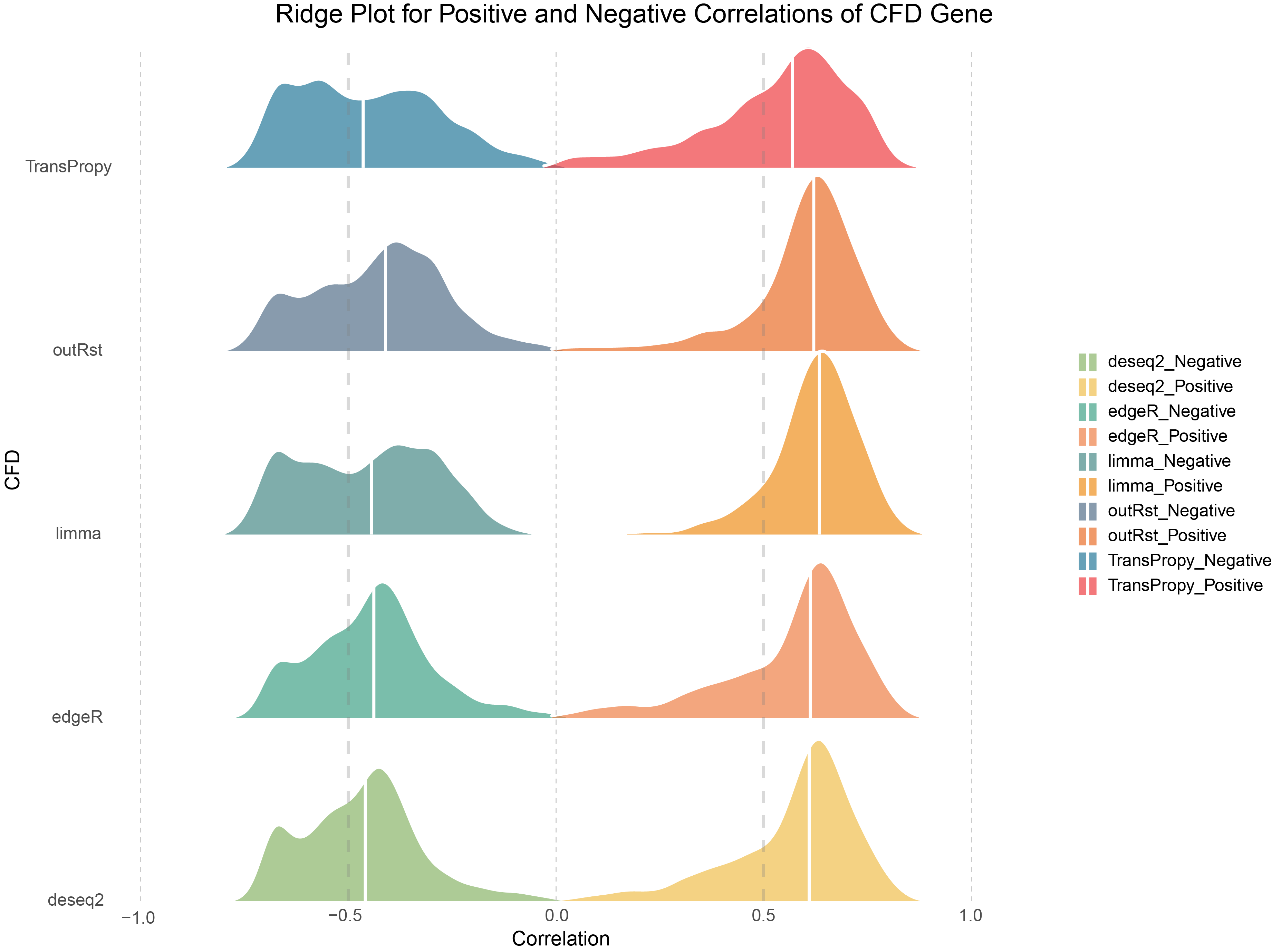
Ridge Plot for Positive and Negative Correlations of CFD Gene
11.8 ANKRD35 Ridge Plot
# Define colors for ANKRD35 Gene
colors <- c("#7b1fa2", "#afb42b", "#512da8", "#fbc02d", "#303f9f", "#ffa000", "#1565c0", "#f57c00", "#0288d1", "#e64a19")

# Plot Ridge Plot for ANKRD35 Gene
ggplot(combined_ANKRD35, aes(x = cor, y = methods, fill = cor_type)) +
  geom_density_ridges(
    alpha = 0.7,
    color = 'white',
    scale = 1,  # Adjust overlap degree, scale = 1 just touches the baseline, larger values increase overlap
    rel_min_height = 0.01,  # Tail trimming, larger values trim more
    quantile_lines = TRUE,
    quantiles = 2,
    linewidth = 1
  ) +
  scale_fill_manual(values = colors) +
  labs(
    title = "Ridge Plot for Positive and Negative Correlations of ANKRD35 Gene",
    x = "Correlation",
    y = "ANKRD35"
  ) +
  theme(
    axis.text.x = element_text(angle = 90, hjust = 1)
  ) +
  geom_vline(
    xintercept = c(-0.5, 0.5),
    linewidth = 1,
    color = 'grey50',
    lty = 'dashed',
    alpha = 0.3
  ) +
  geom_vline(
    xintercept = c(-1, 0, 1),
    linewidth = 0.4,
    color = 'grey',
    lty = 'dashed',
    alpha = 0.8
  ) +
  theme_classic() +
  scale_y_discrete(expand = c(0,0)) +
  theme_minimal() +
  theme(
    panel.grid = element_blank(),
    # axis.text.y = element_blank(),
    legend.title = element_blank()
  )
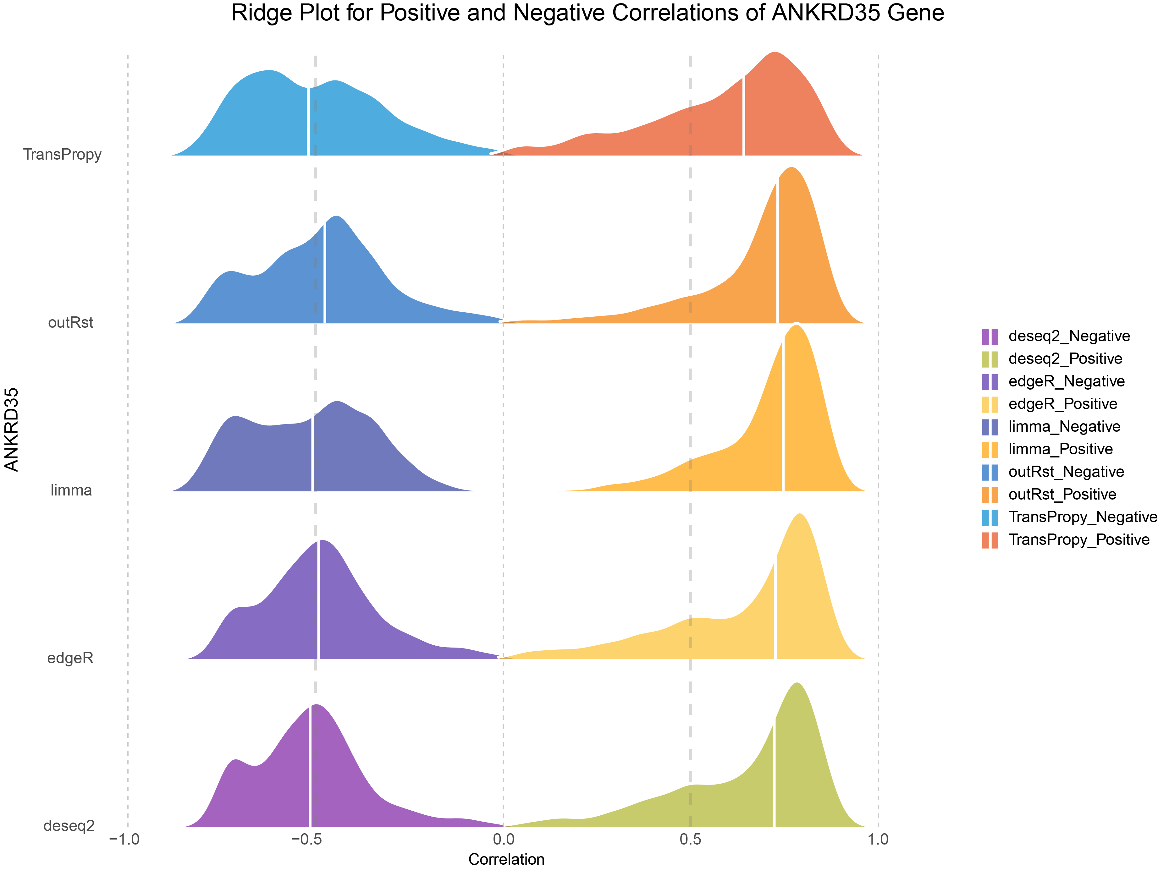
Ridge Plot for Positive and Negative Correlations of ANKRD35 Gene
11.9 ALOXE3 Ridge Plot
# Define colors for ALOXE3 Gene
colors <- c("#00838f", "#c62828", "#00695c", "#ad1457", "#2e7d32", "#6a1b9a", "#558b2f", "#4527a0", "#9e9d24", "#283593")

# Plot Ridge Plot for ALOXE3 Gene
ggplot(combined_ALOXE3, aes(x = cor, y = methods, fill = cor_type)) +
  geom_density_ridges(
    alpha = 0.6,
    color = 'white',
    scale = 1,  # Adjust overlap degree, scale = 1 just touches the baseline, larger values increase overlap
    rel_min_height = 0.01,  # Tail trimming, larger values trim more
    quantile_lines = TRUE,
    quantiles = 2,
    linewidth = 1
  ) +
  scale_fill_manual(values = colors) +
  labs(
    title = "Ridge Plot for Positive and Negative Correlations of ALOXE3 Gene",
    x = "Correlation",
    y = "ALOXE3"
  ) +
  theme(
    axis.text.x = element_text(angle = 90, hjust = 1)
  ) +
  geom_vline(
    xintercept = c(-0.5, 0.5),
    linewidth = 1,
    color = 'grey50',
    lty = 'dashed',
    alpha = 0.3
  ) +
  geom_vline(
    xintercept = c(-1, 0, 1),
    linewidth = 0.4,
    color = 'grey',
    lty = 'dashed',
    alpha = 0.8
  ) +
  theme_classic() +
  scale_y_discrete(expand = c(0,0)) +
  theme_minimal() +
  theme(
    panel.grid = element_blank(),
    # axis.text.y = element_blank(),
    legend.title = element_blank()
  )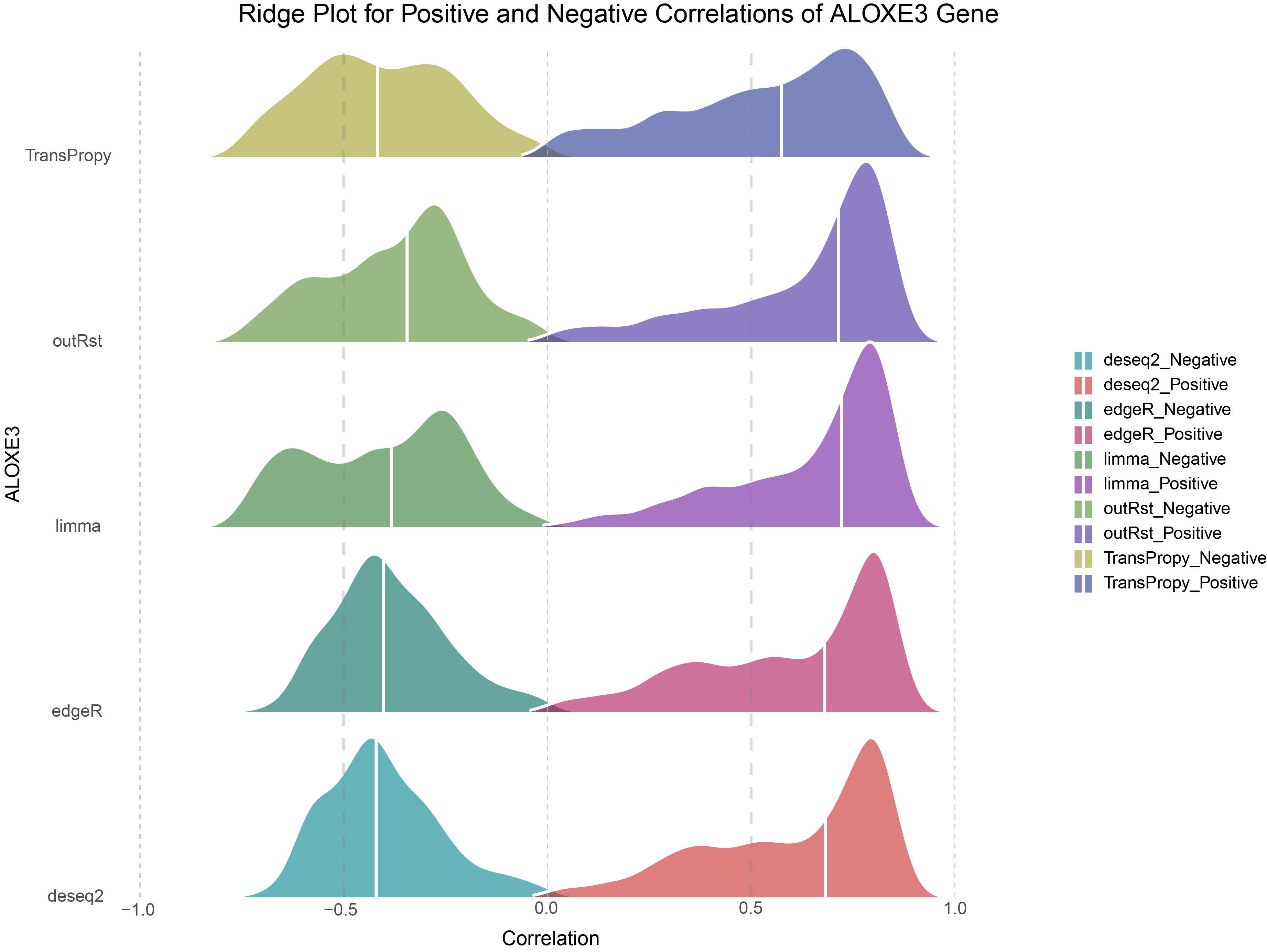
Ridge Plot for Positive and Negative Correlations of ALOXE3 Gene
11.10 Methods
- Finding the top three genes with the highest countdown: CFD, ANKRD35, ALOXE3
- Since the TransPropy method has the most balanced proportion of positively and negatively correlated genes, while other methods have a higher UpRatio than DownRatio, we chose the top three genes with the highest DownRatio in the TransPropy method. This approach will further amplify the difference compared to the other four methods. If the distribution trend remains consistent with the other methods while maintaining its advantage of balanced positive and negative correlations, it suggests that this method has greater potential for practical application.
11.11 Discussion
The data exhibit a bimodal distribution with few low-correlation genes, showing a steep increase on both sides. However, the proportion of Positive genes remains higher than that of Negative genes.
Consistent with the trends observed in DESeq2, edgeR, limma, and outRst methods, the data from the TransPropy method also exhibit a bimodal distribution with few low-correlation genes and a steep increase on both sides. However, compared to these four methods, the TransPropy method shows a more balanced proportion of Positive and Negative genes, with the median distribution being most symmetrically centered around 0 (BEST).
Similar to DESeq2 and edgeR, the data exhibit a bimodal distribution with few low-correlation genes, showing a steep increase on both sides. However, the proportion of Positive genes remains higher than that of Negative genes.